6 Time series

In this section we will learn some basic handling of time series.

This lesson was adapted from Dr. Sam Stevenson’s lecture on Data quality control and outliers: 1D time series and Earth Lab’s Lesson 1. Work With Datetime Format in Python - Time Series Data [1].

About the data

To exemplify some of the basic time series functionalities we will use data about hourly precipitation from four weather stations in the county of Boulder, Colorado from the beginning of 2000 to the end of 2013. In September 2013, an unusual weather pattern led to some of the most intense precipitation ever recorded in this region, causing devastating floods throughout the Colorado Front Range. Our goal is to visualize precipitation data in 2013 and identify this unusual weather event.

Aerial view of floods during September 2013 in Colorado. Photo by State of Colorado.

This data was obtained via the National Oceanic and Atmospheric Administration (NOAA) Climate Data Online service and the resulting CSV can be accessed at this link. The following is a short description of the columns we will work with (the full documentation can be accessed here):

Column	Description
STATION	Identification number identifying the station.
STATION_NAME	Optional field, name identifying the station location.
DATE	this is the year of the record (4 digits), followed by month (2 digits), followed by day of the month (2 digits), followed by a space and ending with a time of observation that is a two digit indication of the local time hour, followed by a colon (:) followed by a two digit indication of the minute which for this dataset will always be 00. Note: The subsequent data value will be for the hour ending at the time specified here. Hour 00:00 will be listed as the first hour of each date, however since this data is by definition an accumulation of the previous 60 minutes, it actually occurred on the previous day.
HPCP	The amount of precipitation recorded at the station for the hour ending at the time specified for DATE above given in inches. The value 999.99 means the data value is missing. Hours with no precipitation are not shown.
Measurement Flag	Left blank when no flag is needed. `[` and `]` mark the beginning and end of a period with missing data, and `{` and `}` mark the beginning and end of a deleted period (the data was received but was unreadable or clearly noise). Rows with these four flags have an HPCP value of 999.99. `g` is only used for day 1 of the month at hour 01:00, when the precipitation amount is zero. Since hours with no precipitation are not shown, almost all rows with an HPCP value of 0 have this flag.

Timestamps

The pandas library represents an instant in time using the pandas.Timestamp class. For example:

import pandas as pd

# Create a timestamp
pd.Timestamp(year=2020,
             month=10,
             day=18,
             hour=12,
             minute=30,
             second=15)

Timestamp('2020-10-18 12:30:15')

When we store multiple pandas.Timestamps in a pandas.Series the data type of the series is set to datetime64[ns]:

# Notice the data type of the series is datetime64
pd.Series([pd.Timestamp(2020, 10, 18),
           pd.Timestamp(2020, 10, 17),
           pd.Timestamp(2020, 10, 16)])

0   2020-10-18
1   2020-10-17
2   2020-10-16
dtype: datetime64[ns]

Data exploration

Let’s start by reading in the data and taking a look at it:

# Read in data
URL = 'https://raw.githubusercontent.com/carmengg/eds-220-book/main/data/boulder_colorado_2013_hourly_precipitation.csv'
precip = pd.read_csv(URL)

precip

	STATION	STATION_NAME	DATE	HPCP	Measurement Flag	Quality Flag
0	COOP:055881	NEDERLAND 5 NNW CO US	20000101 00:00	999.99	]
1	COOP:055881	NEDERLAND 5 NNW CO US	20000101 01:00	0.00	g
2	COOP:055881	NEDERLAND 5 NNW CO US	20000102 20:00	0.00		q
3	COOP:055881	NEDERLAND 5 NNW CO US	20000103 01:00	0.00		q
4	COOP:055881	NEDERLAND 5 NNW CO US	20000103 05:00	0.00		q
...	...	...	...	...	...	...
9001	COOP:050843	BOULDER 2 CO US	20131222 01:00	999.99	[
9002	COOP:050843	BOULDER 2 CO US	20131223 00:00	999.99	]
9003	COOP:050843	BOULDER 2 CO US	20131223 02:00	0.10
9004	COOP:050843	BOULDER 2 CO US	20131229 01:00	999.99	[
9005	COOP:050843	BOULDER 2 CO US	20131231 00:00	999.99	]

9006 rows × 6 columns

Notice the data has records from more than one station. We can check which ones using the unique() method:

# Check which stations are in the data
precip['STATION_NAME'].unique()

array(['NEDERLAND 5 NNW CO US', 'ALLENSPARK 2 SE CO US',
       'LONGMONT 6 NW CO US', 'BOULDER 2 CO US'], dtype=object)

So the data has hourly precipitation records from four stations in Boulder County. The rows are ordered by station first and then by date: all the records from the first station (2000 to 2013), followed by all the records from the second station, and so on. We will come back to this when we use the dates as the index. In this lesson, we will look at the total precipitation over all four stations.

Let’s take an initial look at hour data:

# Plot hourly precipitation from all stations
precip.plot()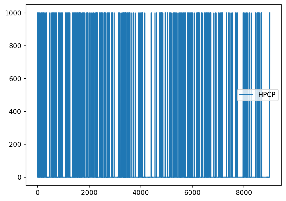

There are a few things going on with this graph:

Outliers: There are many jumps close to 1000. This is clearly not right and these are outliers. Looking at the column descriptions we can see 999.99 indicates the hourly precipitation data is missing.
Indexing: The \(x\)-axis values are given by the index of the data frame and not relative to time.
Time range: We are only interested in the precipitation data from 2013, but this graph is trying to plot all our data.

Let’s fix each one of these issues separately.

Reading in missing data values

The metadata states the missing values are indicated by the number 999.99. We can use this information to reload the data frame indicating 999.99 is the missing value. To do this, we add the na_values parameter to the pandas.read_csv() function to indicate additional values that should be recognized as NA. Since 999.99 only means “missing” in the HPCP column, we pass a dictionary that applies it to that column only:

# Read in CSV indicating NA values in HPCP column based on metadata
precip = pd.read_csv(URL, na_values={'HPCP': [999.99]})

precip.head()

	STATION	STATION_NAME	DATE	HPCP	Measurement Flag	Quality Flag
0	COOP:055881	NEDERLAND 5 NNW CO US	20000101 00:00	NaN	]
1	COOP:055881	NEDERLAND 5 NNW CO US	20000101 01:00	0.0	g
2	COOP:055881	NEDERLAND 5 NNW CO US	20000102 20:00	0.0		q
3	COOP:055881	NEDERLAND 5 NNW CO US	20000103 01:00	0.0		q
4	COOP:055881	NEDERLAND 5 NNW CO US	20000103 05:00	0.0		q

Notice that the first hourly precipitation value used to be 999.99 and it is now set to a NaN. Check the na_values parameter in the pd.read_csv() documentation to learn more about which values are identified as NA by default.

We can try making our plot again:

precip.plot()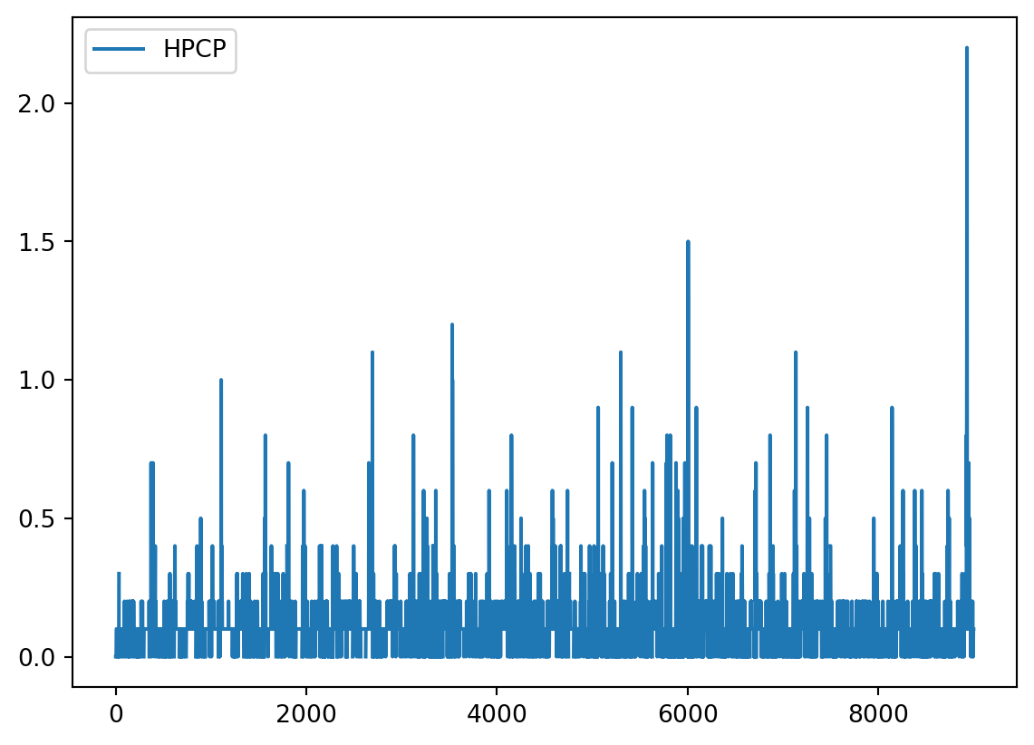

This looks better and we can already see there is something going on close to the end of the time series.

Casting strings into dates

Notice that the DATE column in our data frame is not of type datetime. We can check this using the dtypes attribute for data frames:

# Check whether DATE column is of type datetime
precip.dtypes

STATION              object
STATION_NAME         object
DATE                 object
HPCP                float64
Measurement Flag     object
Quality Flag         object
dtype: object

Remember that the object data type means that (most likely) all values in that column are strings. We can easily convert strings to datetime objects using the pandas.to_datetime() function:

pandas.to_datetime() input: a pandas.Series with strings that can be converted to dates
pandas.to_datetime() output: a pandas.Series with the strings converted to datetime objects

Example

# Preview DATE converted to timestamps
pd.to_datetime(precip['DATE'])

0      2000-01-01 00:00:00
1      2000-01-01 01:00:00
2      2000-01-02 20:00:00
3      2000-01-03 01:00:00
4      2000-01-03 05:00:00
               ...        
9001   2013-12-22 01:00:00
9002   2013-12-23 00:00:00
9003   2013-12-23 02:00:00
9004   2013-12-29 01:00:00
9005   2013-12-31 00:00:00
Name: DATE, Length: 9006, dtype: datetime64[ns]

We can overwrite the DATE column with this output:

# Convert DATE column to timestamps
precip['DATE'] = pd.to_datetime(precip['DATE'])

# Check DATE column data type is updated
print(precip.dtypes)

# Check new values
precip['DATE'].head()

STATION                     object
STATION_NAME                object
DATE                datetime64[ns]
HPCP                       float64
Measurement Flag            object
Quality Flag                object
dtype: object

0   2000-01-01 00:00:00
1   2000-01-01 01:00:00
2   2000-01-02 20:00:00
3   2000-01-03 01:00:00
4   2000-01-03 05:00:00
Name: DATE, dtype: datetime64[ns]

We can make another attempt at plotting our precipitation data:

precip.plot(x='DATE', y='HPCP')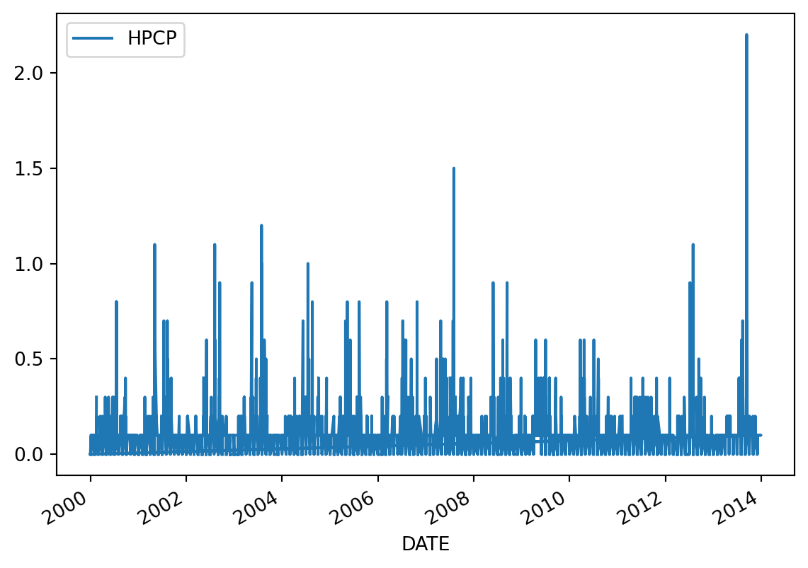

Notice the \(x\)-axis is now neatly organized into years.

Next, using our DATE column as the index will allow us to perform operations with respect to time, including subsetting and resampling. We will also sort the index using sort_index(), so that the rows are in chronological order instead of grouped by station. This will remove some artifacts from our plot. In general, it is good practice to sort a time index, since many time series operations assume the dates are in order.

# Set DATE column as index and sort rows chronologically
precip = precip.set_index('DATE').sort_index()

# Inspect new index
precip.head()

	STATION	STATION_NAME	HPCP	Measurement Flag
DATE
2000-01-01 00:00:00	COOP:055881	NEDERLAND 5 NNW CO US	NaN	]
2000-01-01 01:00:00	COOP:050843	BOULDER 2 CO US	0.0	g
2000-01-01 01:00:00	COOP:055121	LONGMONT 6 NW CO US	0.0	g
2000-01-01 01:00:00	COOP:050183	ALLENSPARK 2 SE CO US	0.0	g
2000-01-01 01:00:00	COOP:055881	NEDERLAND 5 NNW CO US	0.0	g

Since we know the default behavior of plot() is to use the index as the \(x\)-axis and make a line plot for each numeric column, we can simplify our plot making like this:

precip.plot()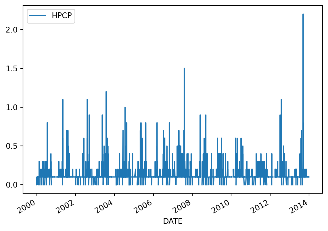

Leverage pandas.read_csv() to set a known index

If we already have information about our data frame and know which column we will use as the index, we can directly set the index when we load the data by using:

df = pandas.read_csv(file, index_col='index_column')

If we also need our index to be of type datetime and we have a known dates column, then we can also create a datetime index directly when loading the data:

df = pandas.read_csv(file, index_col='date_column', parse_dates=['date_column'])

If the rows in the file are not in chronological order, remember to add sort_index() after loading the data.

Subsetting by date

pandas has great functionality to subset a data frame when using a time index.

Example

We can use .loc[year-month] to select data from a specific year and month:

# Select precipitation data from September 2013
precip.loc['2013-09']

	STATION	STATION_NAME	HPCP	Measurement Flag	Quality Flag
DATE
2013-09-01 00:00:00	COOP:055881	NEDERLAND 5 NNW CO US	NaN	]
2013-09-01 00:00:00	COOP:055121	LONGMONT 6 NW CO US	NaN	}
2013-09-01 00:00:00	COOP:050183	ALLENSPARK 2 SE CO US	NaN	]
2013-09-01 01:00:00	COOP:050183	ALLENSPARK 2 SE CO US	NaN	[
2013-09-01 01:00:00	COOP:055881	NEDERLAND 5 NNW CO US	NaN	[
...	...	...	...	...	...
2013-09-27 14:00:00	COOP:055121	LONGMONT 6 NW CO US	0.1
2013-09-27 15:00:00	COOP:050843	BOULDER 2 CO US	0.1
2013-09-27 17:00:00	COOP:050843	BOULDER 2 CO US	0.1
2013-09-27 18:00:00	COOP:050843	BOULDER 2 CO US	0.1
2013-09-27 20:00:00	COOP:055121	LONGMONT 6 NW CO US	0.1

128 rows × 5 columns

Or simply select data from a given year using .loc[year]:

# Select 2013 precipitation data
precip.loc['2013']

	STATION	STATION_NAME	HPCP	Measurement Flag	Quality Flag
DATE
2013-01-01 00:00:00	COOP:050183	ALLENSPARK 2 SE CO US	NaN	]
2013-01-01 01:00:00	COOP:055121	LONGMONT 6 NW CO US	0.0	g
2013-01-01 01:00:00	COOP:050183	ALLENSPARK 2 SE CO US	NaN	[
2013-01-01 01:00:00	COOP:055881	NEDERLAND 5 NNW CO US	0.0	g
2013-01-01 01:00:00	COOP:050843	BOULDER 2 CO US	0.0	g
...	...	...	...	...	...
2013-12-24 18:00:00	COOP:055881	NEDERLAND 5 NNW CO US	0.1
2013-12-28 22:00:00	COOP:055881	NEDERLAND 5 NNW CO US	0.1
2013-12-29 01:00:00	COOP:050843	BOULDER 2 CO US	NaN	[
2013-12-30 04:00:00	COOP:055881	NEDERLAND 5 NNW CO US	0.1
2013-12-31 00:00:00	COOP:050843	BOULDER 2 CO US	NaN	]

662 rows × 5 columns

We can use this selection to plot data as usual. Notice we have a lot of gaps due to missing data:

precip.loc['2013'].plot()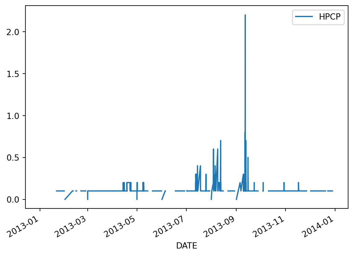

Resample

Resampling a time series means converting a time series from one frequency to another. For example, monthly to yearly (downsampling) or weekly to daily (upsampling). We can resample with the resample() method. The simplest use is to call

df.resample(new_frequency).aggregator_function()

where:

new_frequency is a string representing the new frequency to resample the data, for example 'D' for day, 'W' for week, 'MS' or 'ME' for month start and month end, 'YS' or 'YE' for year start and year end.
aggregator_function() is the function we will use to aggregate the data into the new frequency. For example, max(), min(), sum(), or mean().

The resample() method works similarly to groupby() in the sense that you need to specify a way to aggregate the data to get any output.

Month end or month start?

'ME' stands for “month end” and 'MS' for “month start”. Both group the data by calendar month. The only difference is how each month is labeled: 'ME' uses the last day of the month and 'MS' uses the first day. For example, this is the total monthly precipitation for the first three months of 2013 with each option:

# Monthly totals labeled by the last day of each month
precip.loc['2013', 'HPCP'].resample('ME').sum().head(3)

DATE
2013-01-31    1.0
2013-02-28    2.8
2013-03-31    6.1
Freq: ME, Name: HPCP, dtype: float64

# Monthly totals labeled by the first day of each month
precip.loc['2013', 'HPCP'].resample('MS').sum().head(3)

DATE
2013-01-01    1.0
2013-02-01    2.8
2013-03-01    6.1
Freq: MS, Name: HPCP, dtype: float64

The totals are the same, only the dates in the index change. In this course we will use 'ME'. Similarly, 'YE' and 'YS' label each year by its last or first day.

Example

Our 2013 precipitation data has hourly frequency and we want to resample it to daily frequency.

# Resample 2013 hourly data to daily frequency: no output
precip.loc['2013', 'HPCP'].resample('D')

<pandas.core.resample.DatetimeIndexResampler object at 0x1617a2990>

To get an output we need to add an aggregator function that indicates how we want to summarize the data that falls on each day. In this case we want the total precipitation on a day, so we aggregate it using sum():

# Total daily precipitation in 2013 (sum over all stations)
daily_precip_2013 = precip.loc['2013', 'HPCP'].resample('D').sum()

daily_precip_2013.head(3)

DATE
2013-01-01    0.0
2013-01-02    0.0
2013-01-03    0.0
Freq: D, Name: HPCP, dtype: float64

A few things to notice here:

Each daily value is the total precipitation from all the hourly records on that day, over the four stations.
sum() returns 0 for days without any records. Since hours with no precipitation are not recorded, this is the right value for dry days. A few days only have rows marking missing data, and these also show 0.

The index has now changed to be days in 2013 and, since we selected a single column, the result is a pandas.Series. We should also rename the series since it is no longer hourly precipitation:

# Rename series to match resample
daily_precip_2013 = daily_precip_2013.rename('daily_precipitation')
daily_precip_2013.name

'daily_precipitation'

Finally, we can plot our data:

daily_precip_2013.plot(ylabel='daily precipitation (in)',
                       xlabel='',
                       title='Total precipitation over four stations in Boulder County, CO (2013)')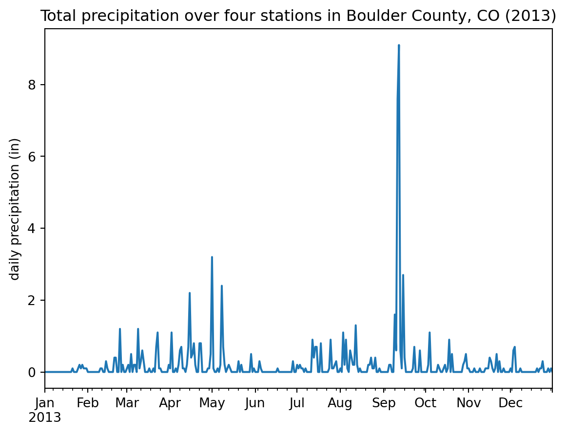

Complete workflow

The previous code includes a lot of exploratory functions and trials. While it is important to keep our data exploration documented, once we are certain of our data wrangling, we can streamline our analyses to only include the code that directly contributes to the output. Moving on, we will start to collect all our relevant code to create such complete workflows. For this lesson, the code below will produce the final graph:

import pandas as pd

# Read in hourly precipitation data from four stations in Boulder County, CO
# HPCP = hourly precipitation (unique numerical column in data frame)
URL = 'https://raw.githubusercontent.com/carmengg/eds-220-book/main/data/boulder_colorado_2013_hourly_precipitation.csv'
precip = (pd.read_csv(URL,
                      na_values={'HPCP': [999.99]},  # Known from metadata
                      index_col='DATE',
                      parse_dates=['DATE'])
          .sort_index()  # Rows in the file are ordered by station
          )


# Calculate daily total precipitation over all stations during 2013
daily_precip_2013 = (precip.loc['2013', 'HPCP']
                            .resample('D')
                            .sum()
                            .rename('daily_precipitation')
                            )

# Plot time series
daily_precip_2013.plot(ylabel='daily precipitation (in)',
                       xlabel='',
                       title='Total precipitation over four stations in Boulder County, CO (2013)')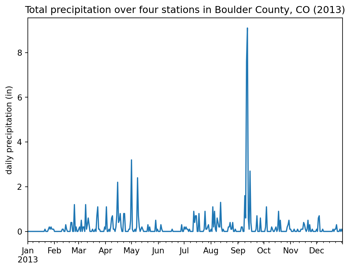

More info

There is so much more to learn about time series data. These resources will allow you to dive deeper:

📖 pandas getting started tutorials - How to handle time series data with ease

📖 Time Series Chapter, Python for Data Analysis, Wes McKinney

📖 pandas User Guide - Time series/date functionality

References

[1]

L. Wasser, N. Korinek, and J. Palomino, “Earthlab/earth-analytics-intermediate-earth-data-science-textbook: Updated ORC ID’s.” Zenodo, Mar. 2024. doi: 10.5281/ZENODO.4683910. Available: https://zenodo.org/doi/10.5281/zenodo.4683910. [Accessed: Oct. 21, 2024]