import numpy as np
import matplotlib.pyplot as plt
import geopandas as gpd
import rioxarray as rioxr

from pystac_client import Client  # To access STAC catalogs

import planetary_computer  # To sign items from the MPC STAC catalog

from IPython.display import Image # To nicely display images15 STAC specification
So far in our course we have obtained data in two ways: by downloading it directly from the data provider or by obtaining a URL from a data repository. This can be a convenient way to access targeted datasets, often usign graphical user interfaces (GUIs) for data discovery and filtering. However, relying on clicking and copy-pasting addresses and file names can make our workflows more error-prone and less reproducible. In particular, satellites around the world produce terabytes of new data daily and manually browsing through data repositories can it make difficult to access this data. Moreover, it can be inconvenient to learn a new way to access data from every single big data provider. This is where STAC comes in.

The SpatioTemporal Asset Catalog (STAC) is an emerging open standard for geospatial data that aims to increase the interoperability of geospatial data, particularly satellite imagery. Many major data archives now follow the STAC specification.
In the next classes we’ll be working with the Microsoft’s Planetary Computer (MPC) STAC API. In this lesson we will learn about the main components of a STAC catalog and how to search for data using the MPC’s STAC API.
Item, collection, and catalog
The STAC item (or just item) is the building block of a STAC. An item is a GeoJSON feature with additional fields that make it easier to find it as we look for data across catalogs.
An item holds two types of information:
Metadata: The metadata for a STAC item includes core identifying information (such as ID, geometry, bounding box, and date), and additional properties (for example, place of collection).
Assets: Assets are links to the actual data of the item (for example, links to the spectral bands of a satellite image.)
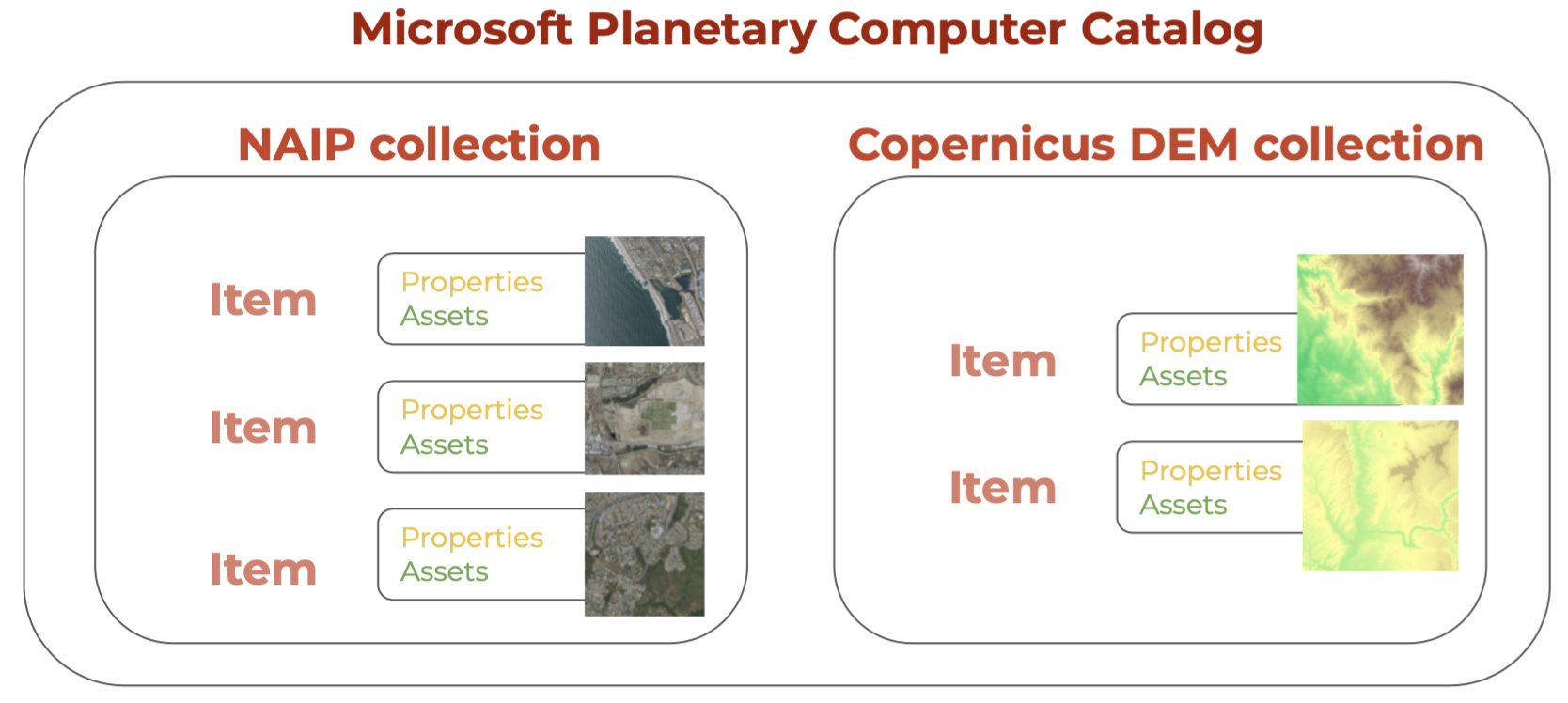
STAC items can be grouped into STAC collections. For example, while a single satellite scene (at a single time and location) would constitue an item, scenes across time and location from the same satellite can be orgnanized in a collection. Finally, multiple collections can be organized into a single STAC catalog.
For example, we’ll be accessing the MPC STAC catalog. Two of its collections are the National Agriculture Imagery Program (NAIP) colelction and the Copernicus Digital Elevation Model (DEM) colleciton. Each of these collections has multiple items, with item cotaining properties (metadata) and assets (links to the data).
Application Programming Interface (API)
To request data from a catalog following the STAC standard we use an Application Programming Interface (API). We can think of an API as an intermediary tasked with sending our request for data to the data catalog and getting the response from the catalog back to us. The following diagram nicely explains what an API does using a real-life analogy of a restaurant:

The Python package to access APIs for STAC catalogs is pystac_client. Our goal in this lesson is to retrieve NAIP data from the MPC’s data catalog via its STAC API.
MPC Catalog
First, load the necessary packages:
Access
We use the Client function from the pystac_client package to access the catalog:
# Access MPC catalog
catalog = Client.open(
    "https://planetarycomputer.microsoft.com/api/stac/v1",
    modifier=planetary_computer.sign_inplace,
)
The modifier parameter is needed to access the data in the MPC catalog.
Catalog Exploration
Let’s check out some of the catalog’s metadata:
# Explore catalog metadata
print('Title:', catalog.title)
print('Description:', catalog.description)
Title: Microsoft Planetary Computer STAC API
Description: Searchable spatiotemporal metadata describing Earth science datasets hosted by the Microsoft Planetary ComputerWe can access its collections by using the get_collections() method:
catalog.get_collections()<generator object Client.get_collections at 0x104d41f10>Notice the output of get_collections() is a generator. This is a special kind of lazy object in Python over which you can loop over like a list. Unlike a list, the items in a generator do not exist in memory until you explicitely iterate over them or convert them to a list. This can allow for more efficient memory allcoation. Once the generator is exhausted (i.e. iterated over completely), it cannot be reused unless it is recreated.
Let’s try getting the collections from the catalog again:
# Get collections and print their names
collections = list(catalog.get_collections())  # Turn generator into list

print('Number of collections:', len(collections))

print("Collections IDs (first 10):")
for i in range(10):
    print('-', collections[i].id)
Number of collections: 126
Collections IDs (first 10):
- daymet-annual-pr
- daymet-daily-hi
- 3dep-seamless
- 3dep-lidar-dsm
- fia
- gridmet
- daymet-annual-na
- daymet-monthly-na
- daymet-annual-hi
- daymet-monthly-hiCollection
The NAIP catalog’s ID is 'naip'. We can select a single collection for exploration using the get_child() method for the catalog and the collection ID as the parameter:
naip_collection = catalog.get_child('naip')
naip_collection
<CollectionClient id=naip>
Catalog search
We can narrow down the search within the catalog by specifying a time range, an area of interest, and the collection name. The simplest ways to define the area of interest to look for data in the catalog are:
- a GeoJSON-type dictionary with the coordinates of the bounding box,
- as a list
[xmin, ymin, xmax, ymax]with the coordinate values defining the four corners of the bounding box.
In this lesson we will look for the NAIP scenes over Santa Barbara from 2018 to 2023. We’ll use the GeoJSON method to define the area of interest:
# Temporal range of interest
time_range = "2018-01-01/2023-01-01"

# NCEAS bounding box (as a GeoJSON)
bbox = {
    "type": "Polygon",
    "coordinates":[
        [
            [-119.70608227128903, 34.426300194372274],
            [-119.70608227128903, 34.42041139020533],
            [-119.6967885126002, 34.42041139020533],
            [-119.6967885126002, 34.426300194372274],
            [-119.70608227128903, 34.426300194372274]
        ]
    ],
}

# Catalog search
search = catalog.search(
    collections = ['naip'],
    intersects = bbox,
    datetime = time_range)
search
<pystac_client.item_search.ItemSearch at 0x153bbcdd0>To get the items found in the search (or check if there were any matches in the search) we use the item_collection() method:
# Retrieve search items
items = search.item_collection()
len(items)3This output tells us there were three items in the catalog that matched our search!
items
<pystac.item_collection.ItemCollection object at 0x15444b450>
Item
Let’s get the first item in the search:
# Get first item in the catalog search
item = items[0]
type(item)pystac.item.ItemRemember the STAC item is the core object in a STAC catalog. The item does not contain the data itself, but rather metadata and assets that contain links to access the actual data. Some of the metadata:
# Print item ID and properties
print('ID:' , item.id)
item.properties
ID: ca_m_3411935_sw_11_060_20220513{'gsd': 0.6,
'datetime': '2022-05-13T16:00:00Z',
'naip:year': '2022',
'proj:bbox': [246930.0, 3806808.0, 253260.0, 3814296.0],
'providers': [{'url': 'https://www.fsa.usda.gov/programs-and-services/aerial-photography/imagery-programs/naip-imagery/',
'name': 'USDA Farm Service Agency',
'roles': ['producer', 'licensor']}],
'naip:state': 'ca',
'proj:shape': [12480, 10550],
'proj:centroid': {'lat': 34.40624, 'lon': -119.71877},
'proj:transform': [0.6, 0.0, 246930.0, 0.0, -0.6, 3814296.0, 0.0, 0.0, 1.0],
'proj:code': 'EPSG:26911'}Just as the item properties, the item assets are given in a dictionary, with each value being a pystac.asset Let’s check the assets in the item:
item.assets{'image': <Asset href=https://naipeuwest.blob.core.windows.net/naip/v002/ca/2022/ca_060cm_2022/34119/m_3411935_sw_11_060_20220513.tif?st=2025-11-23T23%3A51%3A07Z&se=2025-11-25T00%3A36%3A07Z&sp=rl&sv=2025-07-05&sr=c&skoid=9c8ff44a-6a2c-4dfb-b298-1c9212f64d9a&sktid=72f988bf-86f1-41af-91ab-2d7cd011db47&skt=2025-11-24T14%3A25%3A04Z&ske=2025-12-01T14%3A25%3A04Z&sks=b&skv=2025-07-05&sig=xk1U2inYW11OrcsFCvXUjtNEDFsmq2q2NJbEZPxImss%3D>,
'thumbnail': <Asset href=https://naipeuwest.blob.core.windows.net/naip/v002/ca/2022/ca_060cm_2022/34119/m_3411935_sw_11_060_20220513.200.jpg?st=2025-11-23T23%3A51%3A07Z&se=2025-11-25T00%3A36%3A07Z&sp=rl&sv=2025-07-05&sr=c&skoid=9c8ff44a-6a2c-4dfb-b298-1c9212f64d9a&sktid=72f988bf-86f1-41af-91ab-2d7cd011db47&skt=2025-11-24T14%3A25%3A04Z&ske=2025-12-01T14%3A25%3A04Z&sks=b&skv=2025-07-05&sig=xk1U2inYW11OrcsFCvXUjtNEDFsmq2q2NJbEZPxImss%3D>,
'tilejson': <Asset href=https://planetarycomputer.microsoft.com/api/data/v1/item/tilejson.json?collection=naip&item=ca_m_3411935_sw_11_060_20220513&assets=image&asset_bidx=image%7C1%2C2%2C3&format=png>,
'rendered_preview': <Asset href=https://planetarycomputer.microsoft.com/api/data/v1/item/preview.png?collection=naip&item=ca_m_3411935_sw_11_060_20220513&assets=image&asset_bidx=image%7C1%2C2%2C3&format=png>}for key in item.assets.keys():
print(key, '--', item.assets[key].title)image -- RGBIR COG tile
thumbnail -- Thumbnail
tilejson -- TileJSON with default rendering
rendered_preview -- Rendered previewNotice each asset has an href, which is a link to the data. For example, we can use the URL for the 'rendered_preview' asset to plot it:
# Plot rendered preview
Image(url=item.assets['rendered_preview'].href, width=500)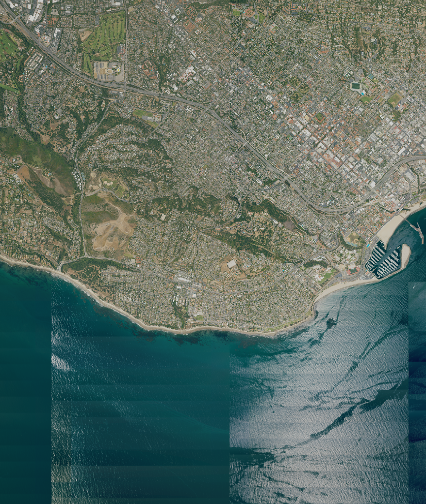
Load data
The raster data in our current item is in the image asset. Again, we access this data via its URL. This time, we open it using rioxr.open_rasterio() directly:
sb = rioxr.open_rasterio(item.assets['image'].href)
sb
<xarray.DataArray (band: 4, y: 12480, x: 10550)> Size: 527MB
[526656000 values with dtype=uint8]
Coordinates:
* band (band) int64 32B 1 2 3 4
* x (x) float64 84kB 2.469e+05 2.469e+05 ... 2.533e+05 2.533e+05
* y (y) float64 100kB 3.814e+06 3.814e+06 ... 3.807e+06 3.807e+06
spatial_ref int64 8B 0
Attributes:
TIFFTAG_IMAGEDESCRIPTION: OrthoVista
TIFFTAG_SOFTWARE: Trimble Germany GmbH
TIFFTAG_XRESOLUTION: 1
TIFFTAG_YRESOLUTION: 1
TIFFTAG_RESOLUTIONUNIT: 1 (unitless)
AREA_OR_POINT: Area
scale_factor: 1.0
add_offset: 0.0Notice this raster has four bands (red, green, blue, nir), so we cannot use the .plot.imshow() method directly (as this function only works when we have three bands). Thus we need select the bands we want to plot (RGB) before plotting:
# Plot raster with correct ratio
size = 6
aspect = sb.rio.width / sb.rio.height
# Select R,G,B bands and plot
sb.sel(band=[1,2,3]).plot.imshow(size=size, aspect=aspect)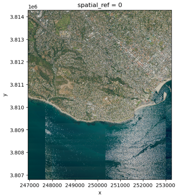
Exercise
The Copernicus Digital Elevation Model (DEM) collection contains elevation data at 90 m spatial resolution. The collection ID in the MPC catalog is 'cop-dem-glo-90'.
- Reuse the
bboxfor Santa Barbara to look for items in this collection. - Get the first item in the search and examine its properties and assets.
- Check the item’s rendered preview asset by clicking on it’s URL.
- Open and plot the item’s data using
rioxarray, save it into a variable nameddem. - Obtain the maximum and minimum elevation on the scene as numbers.
- Print the maximum and minimum elevation rounded to two decimal points using f-strings. For vertical units, consult the data’s handbook.
Aggregation
Let’s take a look at our elevation raster over Santa Barbara:
dem.plot()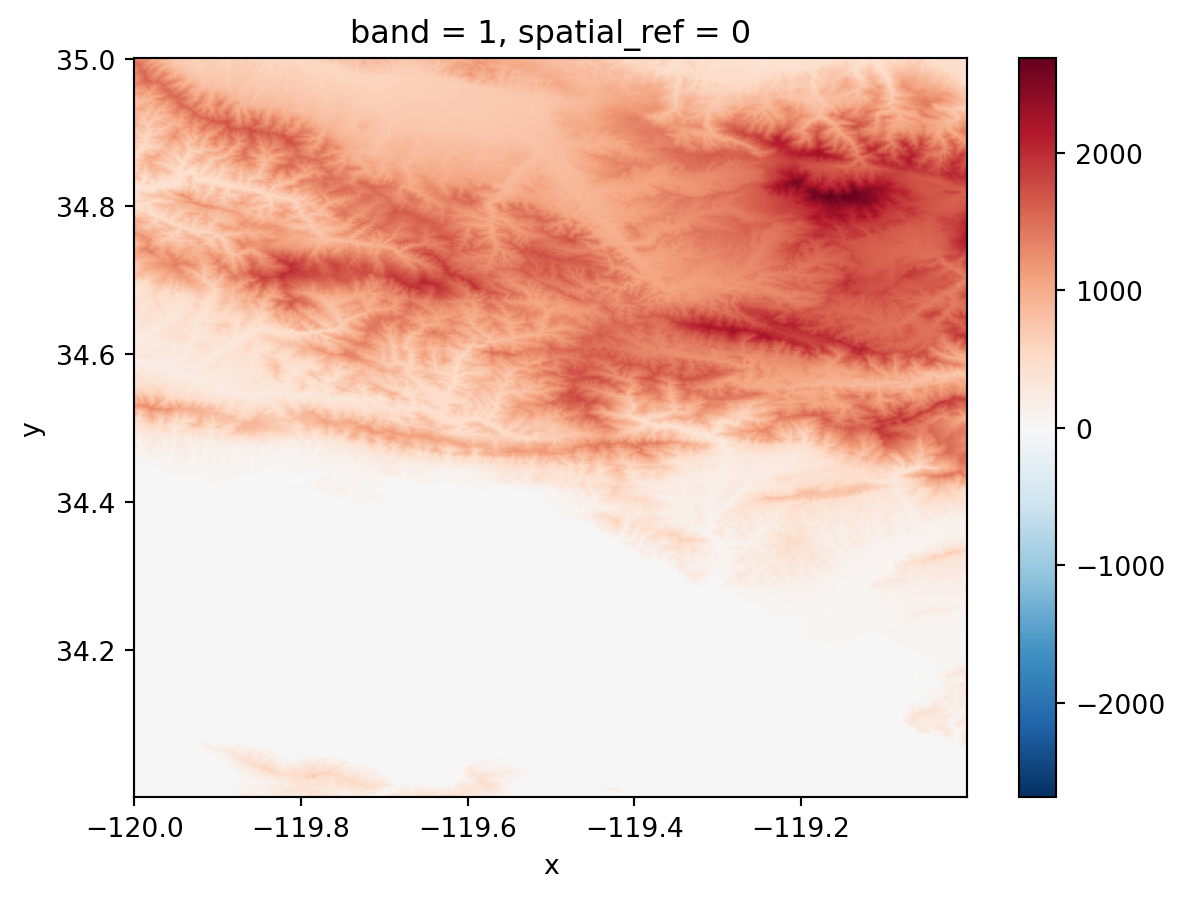
Rasters with high spatial resolution can offer great insight into fine-scale patterns, but can also be challenging to process due to their size.
We can use aggregation methods to spatially downsample a raster into a coarser resolution.
A simple way to spatially downsample an xarray.DataArray is:
xdataarray.coarsen(x=x_window, y=y_window).aggr()where:
xdataarrayis a 2-dimensionalxarray.DataArraywith dimensionsxandy.xandyare the names dimensions of thexarray.DataArray(these could have other names likelon/lat)x_windowandy_windoware the dimensions of the window used to make the aggregation (must be an integer).aggr()is an aggregator function, this is the function which will be applied to each window. Examples aremin(),max(),sum()andmean().
Example
Suppose we want to coarsen our DEM elevation raster from 1200x1200 pixels to a raster of 60x60 pixels by calculating the maximun at each window. Remember the windows are non-overlapping, so we will obtain one pixel per window. A quick division tells us that to got from 1200x1200 to 60x60 we will need to use a 20x20 window. The aggregator function on each of this window will be max().
Our call looks like this:
# Coarsen to a 60x60 raster calculating the maximum value in each window
dem_coarse = dem.coarsen(x=20,y=20).max()
dem_coarse
<xarray.DataArray (band: 1, y: 60, x: 60)> Size: 14kB
array([[[1507.5085 , 1369.9564 , 1120.8246 , ...,  682.03357,
          579.2793 ,  534.9269 ],
        [1579.6641 , 1562.8054 , 1424.9618 , ...,  937.8373 ,
          853.7289 ,  666.9444 ],
        [1476.4916 , 1482.5118 , 1544.5358 , ..., 1194.9047 ,
         1185.6924 ,  950.8014 ],
        ...,
        [   0.     ,    0.     ,    0.     , ...,    0.     ,
            0.     ,    0.     ],
        [   0.     ,    0.     ,    0.     , ...,    0.     ,
            0.     ,    0.     ],
        [   0.     ,    0.     ,    0.     , ...,    0.     ,
            0.     ,    0.     ]]], dtype=float32)
Coordinates:
* band (band) int64 8B 1
* x (x) float64 480B -120.0 -120.0 -120.0 ... -119.0 -119.0 -119.0
* y (y) float64 480B 34.99 34.98 34.96 34.94 ... 34.04 34.03 34.01
spatial_ref int64 8B 0
Attributes:
AREA_OR_POINT: Point
scale_factor: 1.0
add_offset: 0.0# Inspect old and coarsened resolution
print(f"old resolution: {dem.rio.width}x{dem.rio.height}")
print(f"coarse resolution: {dem_coarse.rio.width}x{dem_coarse.rio.height}")
dem_coarse.plot()old resolution: 1200x1200
coarse resolution: 60x60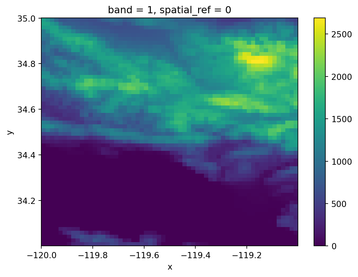
Exercise
- Downsample the elevation raster into a 240x240 raster by taking the average over windows of the appropriate size. Plot the resulting raster.
- Use an f-string to check whether the spatial bounds of the rasters have changed.
- If you are curious about the different colormaps, check out the
xarray documentation.
References
STAC Documentation: